Plotting proportional data as nested circles in R
For better or worse, you see proportional data represented with nested circles a fair bit in the media.
It’s rare that plotting proportional data is not best done with some kind of bar chart, but occasionally I do come across a case where I think nested circles convey a message well (while being visually attractive).
Here I’ll demonstrate how to make a static nested circle plot using the
R package packcircles and ggplot2, although if you want
interactivity you can also check out
circlepackeR which
creates snazzy html widgets.
Packing circles
In the first place, you need a dataframe with the total and subset values you want to plot.
Here is some data I scraped off MycoCosm showing the number of genome assemblies available for different fungal lifestyles, which will be my larger circles. I then want the nested circle area to represent the subset of the total which have already been published - this is actually similar to a figure I created for my PhD thesis introduction!
head(mycocosm.lifestyles.df)
##       lifestyle num num.pub  colour
## 1     endophyte 142      85 #009E73
## 2    lichenised  16       8 #E69F00
## 3  mycoparasite 105      32 #F0E442
## 4   mycorrhizal 199     123 #56B4E9
## 5 phytopathogen 263     155 dimgrey
## 6    saprotroph 258     178 #0072B2
packcircles handles the creation of circles with area proportional to
the numbers we give it.
This involves first generating a dataframe with the central point and radius of each circle.
library(packcircles)

#Get radius and x and y coordinates for centre of larger circles
circle.layout <- circleProgressiveLayout(mycocosm.lifestyles.df$num,
                                         sizetype="area")

#Optionally add a small gap between circles so they're not touching
circle.layout$radius <- circle.layout$radius * 0.95

head(circle.layout)
##           x          y   radius
## 1 -6.723095   0.000000 6.386940
## 2  2.256758   0.000000 2.143920
## 3  2.875424  -8.014137 5.492162
## 4  3.958529  10.072890 7.560930
## 5 16.394459  -1.676497 8.692137
## 6 -9.972836 -15.447186 8.609115
We can then generate a dataframe with enough vertices to plot a polygon that looks like a circle.
#Create a dataframe of vertices to draw each 'circle'
circle.vertices <- circleLayoutVertices(circle.layout, npoints=50)

head(circle.vertices)
##            x         y id
## 1 -0.3361547 0.0000000  1
## 2 -0.3865177 0.8004959  1
## 3 -0.5368122 1.5883674  1
## 4 -0.7846681 2.3511895  1
## 5 -1.1261766 3.0769318  1
## 6 -1.5559518 3.7541492  1
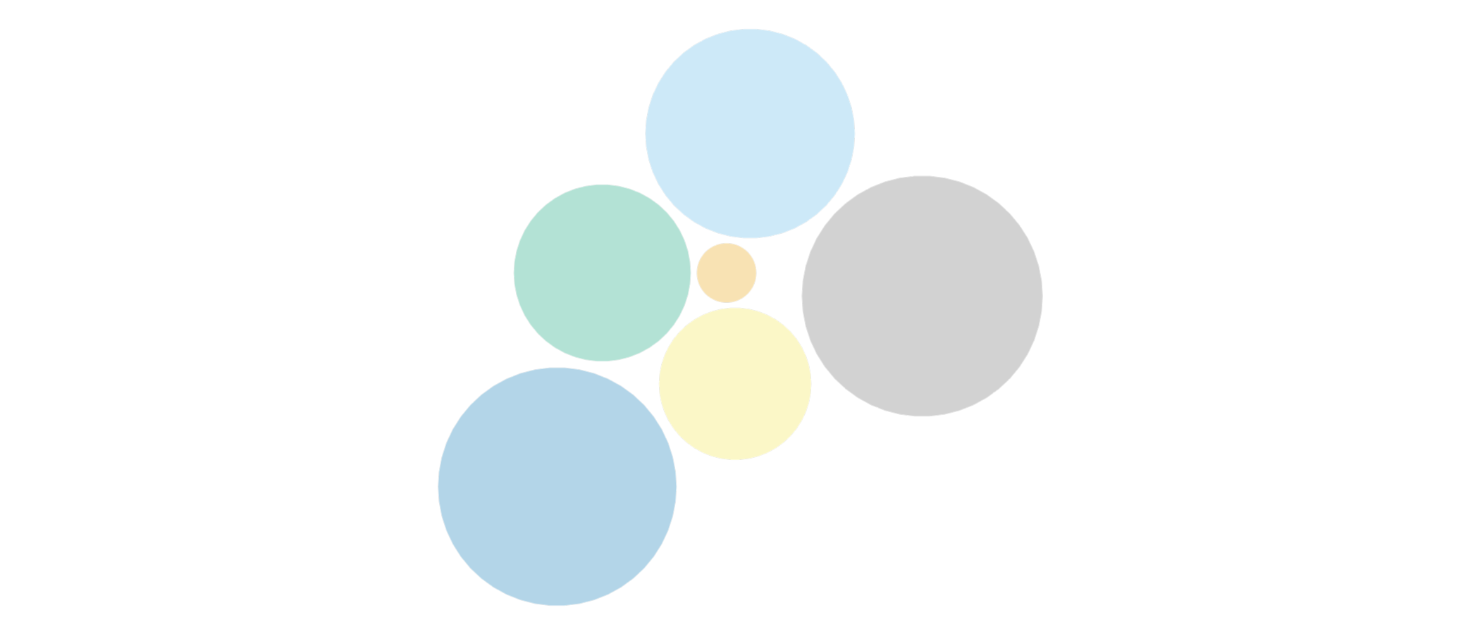
And finally plot the larger circles - we’ll use alpha to make them translucent so that they are distinguished from the nested circles we add later.
library(ggplot2)
library(tgutil)

#Plot circles
gg.circles <- ggplot() +
  geom_polygon(data=circle.vertices,
               aes(x, y, group=id, fill=as.factor(id)),
               colour=NA,
               alpha=0.3) +
  scale_fill_manual(values=mycocosm.lifestyles.df$colour) +
  coord_equal() +
  theme_void() +
  theme(legend.position="none") +
  ggpreview(width=4, height=3, unit="in")
Add nested circles
Now we want to create the polygons for the nested circles, which essentially means repeating the above steps with the nested data.
#Get radius and x and y coordinates for centre of nested circles
circle.layout.pub <-
  circleProgressiveLayout(mycocosm.lifestyles.df$num.pub,
                          sizetype="area")

#If you previously added a small gap between circles, make sure to
#do so again
circle.layout.pub$radius <- circle.layout.pub$radius * 0.95
However before creating the polygon vertices for these nested circles, we first need to replace the central points with those of the larger circles so that our nested ones overlay correctly.
#Replace x and y with that of the larger circles, but keep the
#same radius
circle.layout.pub <- data.frame(x=circle.layout$x,
                                y=circle.layout$y,
                                radius=circle.layout.pub$radius)
Now we can generate the vertices and add the nested circles to the plot.
#Create a dataframe of vertices to draw each nested 'circle'
circle.vertices.pub <- circleLayoutVertices(circle.layout.pub,
											npoints=50)

#Add to plot
gg.circles.nested <- gg.circles +
  geom_polygon(data=circle.vertices.pub,
               aes(x, y, group=id, fill=as.factor(id)),
               colour=NA) +
  ggpreview(width=4, height=3, unit="in")

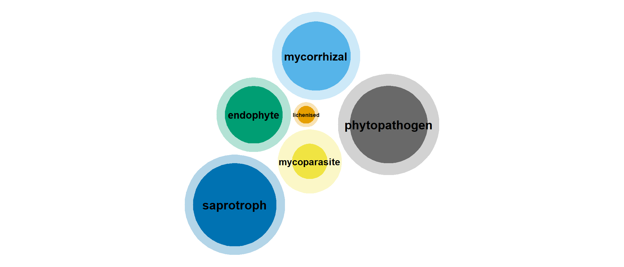
Add labels
Finally we can make another dataframe with information to label the circles.
#Combine original dataframe with the layout dataframe
circle.labels <- cbind(mycocosm.lifestyles.df, circle.layout)

#Add lifestyle labels to centre of circles
gg.circles.nested +
  geom_text(data=circle.labels,
            aes(x, y, size=num, label=lifestyle),
            fontface="bold") +
  scale_size_continuous(range=c(1.5, 3.5))
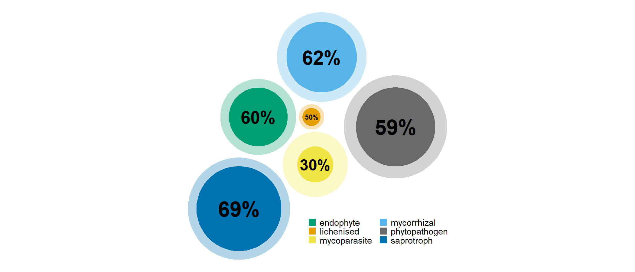
Alternatively we could label with the original values or percentage published, and add a colour legend for the lifestyles.
#Add new column with percentage of published genomes
circle.labels$percent <- round(
  circle.labels$num.pub/circle.labels$num * 100
  )

#Add percentage labels
gg.circles.nested +
  geom_text(data=circle.labels,
            aes(x, y, size=num, label=paste0(percent, "%")),
            fontface="bold",
            show.legend=FALSE) +
  scale_size_continuous(range=c(2, 6)) +
  scale_fill_manual(values=circle.labels$colour,
                    labels=circle.labels$lifestyle) +
  guides(fill=guide_legend(
    nrow=3,
    direction="horizontal",
    title=NULL,
    label.theme=element_text(size=7, margin=margin(l=-3)),
    keywidth=unit(7, "pt"),
    keyheight=unit(7, "pt"))
  ) +
  theme(legend.position=c(0.7, 0.15))
Pretty simple!
Session details
sessionInfo()
## R version 4.2.2 (2022-10-31 ucrt)
## Platform: x86_64-w64-mingw32/x64 (64-bit)
## Running under: Windows 10 x64 (build 22621)
##
## Matrix products: default
##
## locale:
## [1] LC_COLLATE=English_United Kingdom.utf8
## [2] LC_CTYPE=English_United Kingdom.utf8
## [3] LC_MONETARY=English_United Kingdom.utf8
## [4] LC_NUMERIC=C
## [5] LC_TIME=English_United Kingdom.utf8
##
## attached base packages:
## [1] stats     graphics  grDevices utils     datasets  methods   base
##
## other attached packages:
## [1] tgutil_0.1.14     ggplot2_3.4.2     packcircles_0.3.5
##
## loaded via a namespace (and not attached):
##  [1] Rcpp_1.0.9        highr_0.10        pillar_1.9.0      compiler_4.2.2
##  [5] tools_4.2.2       digest_0.6.31     evaluate_0.21     lifecycle_1.0.3
##  [9] tibble_3.2.1      gtable_0.3.3      png_0.1-8         pkgconfig_2.0.3
## [13] rlang_1.1.1       cli_3.6.0         rstudioapi_0.14   yaml_2.3.6
## [17] xfun_0.36         fastmap_1.1.0     withr_2.5.0       dplyr_1.1.2
## [21] knitr_1.42        generics_0.1.3    vctrs_0.6.2       systemfonts_1.0.4
## [25] grid_4.2.2        tidyselect_1.2.0  glue_1.6.2        R6_2.5.1
## [29] textshaping_0.3.6 fansi_1.0.3       rmarkdown_2.21    farver_2.1.1
## [33] magrittr_2.0.3    scales_1.2.1      htmltools_0.5.4   colorspace_2.0-3
## [37] labeling_0.4.2    ragg_1.2.5        utf8_1.2.2        munsell_0.5.0