Marking telomeres on a simple ideogram in R
I was recently running the telomere identifier Tapestry on some genome assemblies to assess how close they were to chromosome-level. Tapestry already outputs an ideogram of assembly scaffolds marked with telomeres, but I wanted to customise the plot to make it clearer when showing collaborators.
There are a couple of R packages that can produce ideograms, including karyoploteR and ggbio, both of which I’ve dabbled in. But in this case I really wanted something even simpler than what either of those packages offer, and instead made a very basic telomere-marked ideogram using just ggplot2.
Basic ideogram
For the absolute simplest plot, the tsv produced during a Tapestry run contains all the information needed.
#Read in tapestry output file
tapestry <- read.csv("contig_details.tsv", sep="\t")

library(tidyverse)

tapestry %>%
  select(Contig, Length, GC., StartTelomeres, EndTelomeres) %>%
  slice_head(n=10)
##       Contig  Length  GC. StartTelomeres EndTelomeres
## 1 scaffold_1 7084357 51.3              0           18
## 2 scaffold_2 6698278 51.1             20           20
## 3 scaffold_3 6429383 50.1              0           18
## 4 scaffold_4 5545257 51.1              2            0
## 5 scaffold_5 3905873 50.3              0           13
## 6 scaffold_6 3299090 50.9             21           17
## 7 scaffold_7 1474513 49.5             22            0
## 8 scaffold_8  834656 48.0             16            6
## 9 scaffold_9   21427 32.6              0            1
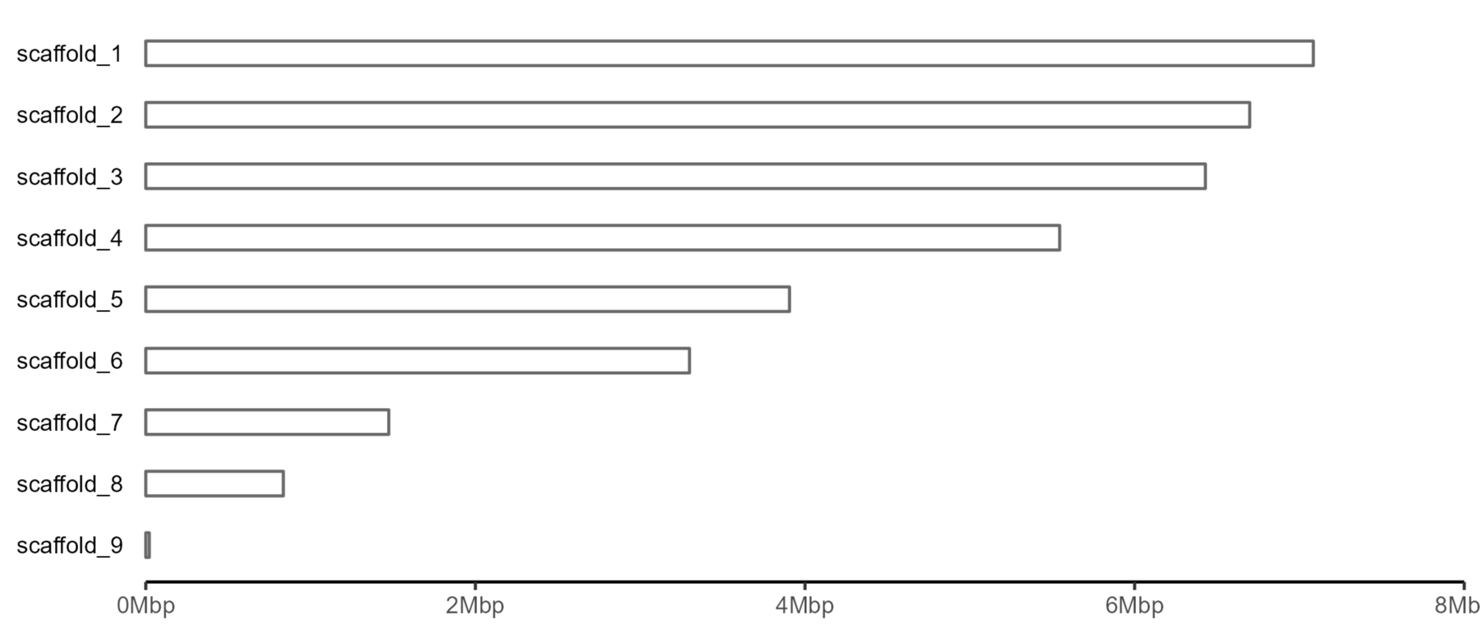
We can then use geom_rect to plot the scaffolds.
#Make sure the scaffolds are ordered from largest to smallest for
#plotting
tapestry$Contig <- factor(
  tapestry$Contig,
  levels=tapestry$Contig[order(tapestry$Length, decreasing=FALSE)]
)

library(ggplot2)
library(scales)
library(tgutil)

#Plot ideograms
gg.ideogram <- ggplot(tapestry, aes(x=Contig, y=Length)) +
  geom_rect(aes(ymax=Length),
            ymin=1,
            xmin=as.numeric(tapestry$Contig)-0.2,
            xmax=as.numeric(tapestry$Contig)+0.2,
            fill="white",
            colour="dimgrey") +
  scale_y_continuous(
    limits=c(0, ceiling(max(tapestry$Length)/1e6)*1e6),
    labels=label_number(
      accuracy=1,
      scale=1e-6,
      suffix="Mbp"),
    expand=c(0, 100)
  ) +
  coord_flip(clip="off") +
  theme(axis.text.y=element_text(
    colour="black",
    size=8,
    margin=margin(r=5)
  ),
  axis.text.x=element_text(size=8),
  axis.ticks.y=element_blank(),
  axis.title=element_blank(),
  axis.line.x=element_line(),
  panel.grid.major=element_blank(),
  panel.grid.minor=element_blank(),
  panel.background=element_blank()) +
  ggpreview(width=7, height=3, units="in")
Now we need to make an additional dataframe with telomere positions.
#Restructure dataframe for plotting
telomeres <- tapestry %>%
  gather(telomere, num.telomeres, StartTelomeres, EndTelomeres)
#Replace 0 telomeres with NA
telomeres$num.telomeres[telomeres$num.telomeres == 0] <- NA

#Add positions for start and end of scaffolds
telomeres$y.pos <- ifelse(
  telomeres$telomere == "StartTelomeres", 1, telomeres$Length
)
We can then add the telomeres to the scaffolds using geom_segment.
#Add telomeres to ideogram
gg.ideogram.telomeres <- gg.ideogram +
  geom_segment(data=telomeres,
               aes(y=y.pos,
                   yend=y.pos,
                   colour=num.telomeres),
               x=as.numeric(telomeres$Contig)-0.3,
               xend=as.numeric(telomeres$Contig)+0.3,
               size=0.7) +
  scale_y_continuous(labels=label_number(accuracy=1,
                                         scale=1e-6,
                                         suffix="Mbp"),
                     expand=c(0, 100)) +
  scale_colour_gradient(
    name="Number of telomeric repeats",
    limits=c(1, max(na.omit(telomeres$num.telomeres))),
    low="#ffbdbd", high="#ff0000", na.value="transparent"
  ) +
  guides(colour=guide_colourbar(
    title.position="top",
    title.theme=element_text(face="bold", size=8))
  ) +
  theme(legend.position=c(0.8, 0.2),
        legend.direction="horizontal",
        legend.text=element_text(size=7),
        legend.key.size=unit(0.5, "cm"),
        legend.margin=margin(0, 0, 0, 0, unit="pt")) +
  ggpreview(width=7, height=3, units="in")
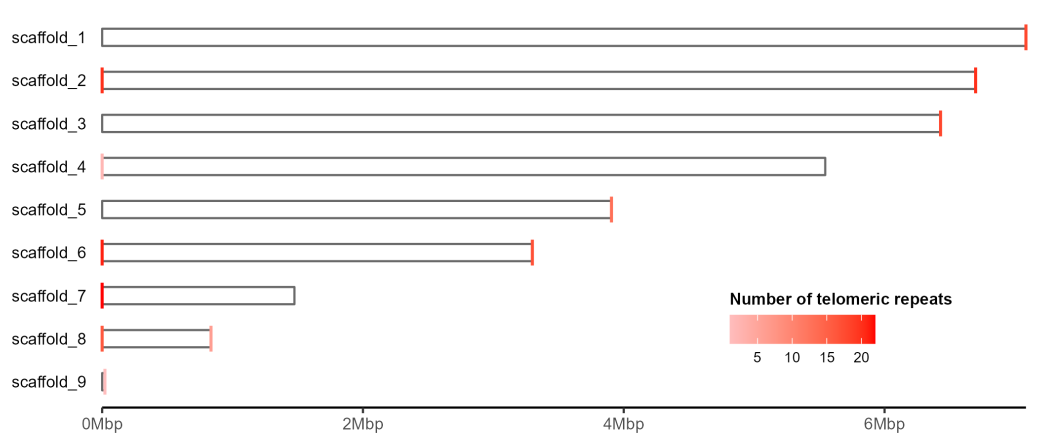
The plot produced by Tapestry colours telomeres opaque red if there are more than 20 repeats detected at the scaffold end, and semi-transparent if up to 20 are detected. Here I’ve opted to use a continuous gradient, but this could easily be modified depending on preference.
Using a gff3
Alternatively, if we have already annotated the genome and want to further customise the ideogram, we can read in the gff3 file.
library(rtracklayer)

#Import the annotation
annotation <- import("Gnomoniopsis_smithogilvyi_IMI355082.gff3")

as.data.frame(annotation) %>%
  select(seqnames, start, end, type, ID, Name) %>%
  slice_head(n=10)
##      seqnames start   end type                    ID Name
## 1  scaffold_1 16179 17332 gene          N0V93_000001 <NA>
## 2  scaffold_1 16179 17332 mRNA       N0V93_000001-T1 <NA>
## 3  scaffold_1 16179 16744 exon N0V93_000001-T1.exon1 <NA>
## 4  scaffold_1 16851 17257 exon N0V93_000001-T1.exon2 <NA>
## 5  scaffold_1 17307 17332 exon N0V93_000001-T1.exon3 <NA>
## 6  scaffold_1 16179 16744  CDS   N0V93_000001-T1.cds <NA>
## 7  scaffold_1 16851 17257  CDS   N0V93_000001-T1.cds <NA>
## 8  scaffold_1 17307 17332  CDS   N0V93_000001-T1.cds <NA>
## 9  scaffold_1 18689 20177 gene          N0V93_000002 <NA>
## 10 scaffold_1 18689 20177 mRNA       N0V93_000002-T1 <NA>
For instance, we may want to only plot scaffolds which actually have gene models on them, and so can filter out the other scaffolds before plotting - in this case nothing changes as all our scaffolds have gene models on them!
#Filter out scaffolds with no annotated gene models
tapestry <-
  tapestry[tapestry$Contig %in% levels(seqnames(annotation)),]
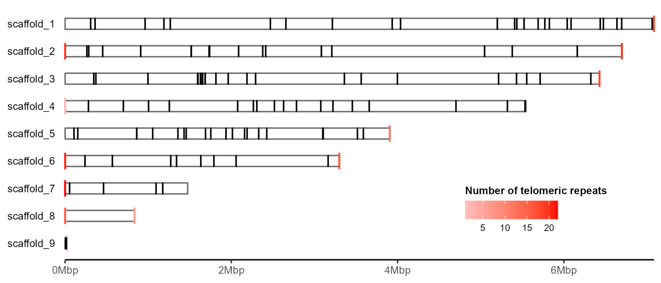
If we have the gff we can also add certain features to the ideogram.
#Make dataframe with start and end positions for tRNAs
tRNAs <- as.data.frame(annotation) %>%
  filter(type == "tRNA") %>%
  mutate(seqnames=factor(seqnames, levels=levels(tapestry$Contig)))

#Add tRNA positions
gg.ideogram.telomeres.trnas <- gg.ideogram.telomeres +
  geom_rect(data=tRNAs,
            aes(ymin=start, ymax=end),
            fill="grey",
            colour="black",
            xmin=as.numeric(tRNAs$seqnames)-0.2,
            xmax=as.numeric(tRNAs$seqnames)+0.2,
            inherit.aes=FALSE) +
  ggpreview(width=7, height=3, units="in")
Or choose to highlight a specific gene.
#Make dataframe with start and end positions for RPB gene family members
genes <- as.data.frame(annotation) %>%
  filter(grepl("^RPB", Name)) %>%
  mutate(seqnames=factor(seqnames, levels=levels(tapestry$Contig)))

#Add gene positions with labels
gg.ideogram.telomeres.genes <- gg.ideogram.telomeres +
  geom_rect(data=genes,
            aes(ymin=start, ymax=end, fill=product),
            xmin=as.numeric(genes$seqnames)-0.2,
            xmax=as.numeric(genes$seqnames)+0.2,
            fill="grey",
            colour="black",
            inherit.aes=FALSE) +
  geom_label(data=genes,
             aes(label=Name, y=(start+end)/2),
             x=as.numeric(genes$seqnames)+0.5,
             label.size=NA,
             fontface="bold",
             fill="dimgrey",
             colour="white",
             size=2,
             label.padding=unit(2, "pt"),
             inherit.aes=FALSE) +
  ggpreview(width=7, height=3, units="in")

Of course, with all the excellent ggplot functions out there the sky’s the limit for how you could choose to customise these plots!
Session details
sessionInfo()
## R version 4.2.2 (2022-10-31 ucrt)
## Platform: x86_64-w64-mingw32/x64 (64-bit)
## Running under: Windows 10 x64 (build 22621)
##
## Matrix products: default
##
## locale:
## [1] LC_COLLATE=English_United Kingdom.utf8
## [2] LC_CTYPE=English_United Kingdom.utf8
## [3] LC_MONETARY=English_United Kingdom.utf8
## [4] LC_NUMERIC=C
## [5] LC_TIME=English_United Kingdom.utf8
##
## attached base packages:
## [1] stats4    stats     graphics  grDevices utils     datasets  methods
## [8] base
##
## other attached packages:
##  [1] rtracklayer_1.58.0   GenomicRanges_1.50.2 GenomeInfoDb_1.34.9
##  [4] IRanges_2.32.0       S4Vectors_0.36.2     BiocGenerics_0.44.0
##  [7] tgutil_0.1.14        scales_1.2.1         forcats_0.5.2
## [10] stringr_1.5.0        dplyr_1.0.10         purrr_1.0.1
## [13] readr_2.1.3          tidyr_1.2.1          tibble_3.1.8
## [16] ggplot2_3.4.0        tidyverse_1.3.2
##
## loaded via a namespace (and not attached):
##  [1] matrixStats_0.63.0          bitops_1.0-7
##  [3] fs_1.5.2                    lubridate_1.9.0
##  [5] httr_1.4.4                  tools_4.2.2
##  [7] backports_1.4.1             utf8_1.2.2
##  [9] R6_2.5.1                    DBI_1.1.3
## [11] colorspace_2.0-3            withr_2.5.0
## [13] tidyselect_1.2.0            compiler_4.2.2
## [15] Biobase_2.58.0              textshaping_0.3.6
## [17] cli_3.6.0                   rvest_1.0.3
## [19] xml2_1.3.3                  DelayedArray_0.23.2
## [21] labeling_0.4.2              systemfonts_1.0.4
## [23] digest_0.6.31               Rsamtools_2.14.0
## [25] rmarkdown_2.19              XVector_0.38.0
## [27] pkgconfig_2.0.3             htmltools_0.5.4
## [29] MatrixGenerics_1.10.0       dbplyr_2.3.0
## [31] fastmap_1.1.0               highr_0.10
## [33] rlang_1.0.6                 readxl_1.4.1
## [35] rstudioapi_0.14             BiocIO_1.8.0
## [37] farver_2.1.1                generics_0.1.3
## [39] jsonlite_1.8.4              BiocParallel_1.32.5
## [41] googlesheets4_1.0.1         RCurl_1.98-1.10
## [43] magrittr_2.0.3              GenomeInfoDbData_1.2.9
## [45] Matrix_1.5-1                munsell_0.5.0
## [47] fansi_1.0.3                 lifecycle_1.0.3
## [49] stringi_1.7.12              yaml_2.3.6
## [51] SummarizedExperiment_1.28.0 zlibbioc_1.44.0
## [53] grid_4.2.2                  parallel_4.2.2
## [55] crayon_1.5.2                lattice_0.20-45
## [57] Biostrings_2.66.0           haven_2.5.1
## [59] hms_1.1.2                   knitr_1.41
## [61] pillar_1.8.1                rjson_0.2.21
## [63] codetools_0.2-18            reprex_2.0.2
## [65] XML_3.99-0.13               glue_1.6.2
## [67] evaluate_0.19               modelr_0.1.10
## [69] png_0.1-8                   vctrs_0.5.1
## [71] tzdb_0.3.0                  cellranger_1.1.0
## [73] gtable_0.3.1                assertthat_0.2.1
## [75] xfun_0.36                   broom_1.0.2
## [77] restfulr_0.0.15             ragg_1.2.5
## [79] googledrive_2.0.0           gargle_1.2.1
## [81] GenomicAlignments_1.34.0    timechange_0.2.0
## [83] ellipsis_0.3.2